DBSCAN Scikit-Learn Tutorial: Clustering with Noise and Arbitrary Shapes
Introduction
DBSCAN Scikit-Learn: In data science and machine learning, clustering is an essential technique for grouping data points into meaningful clusters based on their similarities. Among the many clustering algorithms, DBSCAN (Density-Based Spatial Clustering of Applications with Noise) stands out for its ability to discover clusters of arbitrary shapes and effectively handle noise. This sets it apart from algorithms like K-Means, which rely on spherical clusters and require pre-defining the number of clusters.
In this guide, we will explore DBSCAN using Scikit-Learn, covering its fundamentals, practical implementation, parameter tuning, real-world use cases, and limitations. By the end, you will understand how to utilize DBSCAN Scikit-Learn to reveal hidden patterns in complex datasets.
What is DBSCAN?
DBSCAN Scikit-Learn is a density-based clustering algorithm designed to identify clusters based on the density of data points. It works by defining regions of high density (clusters) separated by regions of low density (noise). Unlike K-Means, DBSCAN Scikit-Learn does not require specifying the number of clusters in advance, making it more flexible for exploratory data analysis.
How DBSCAN Works
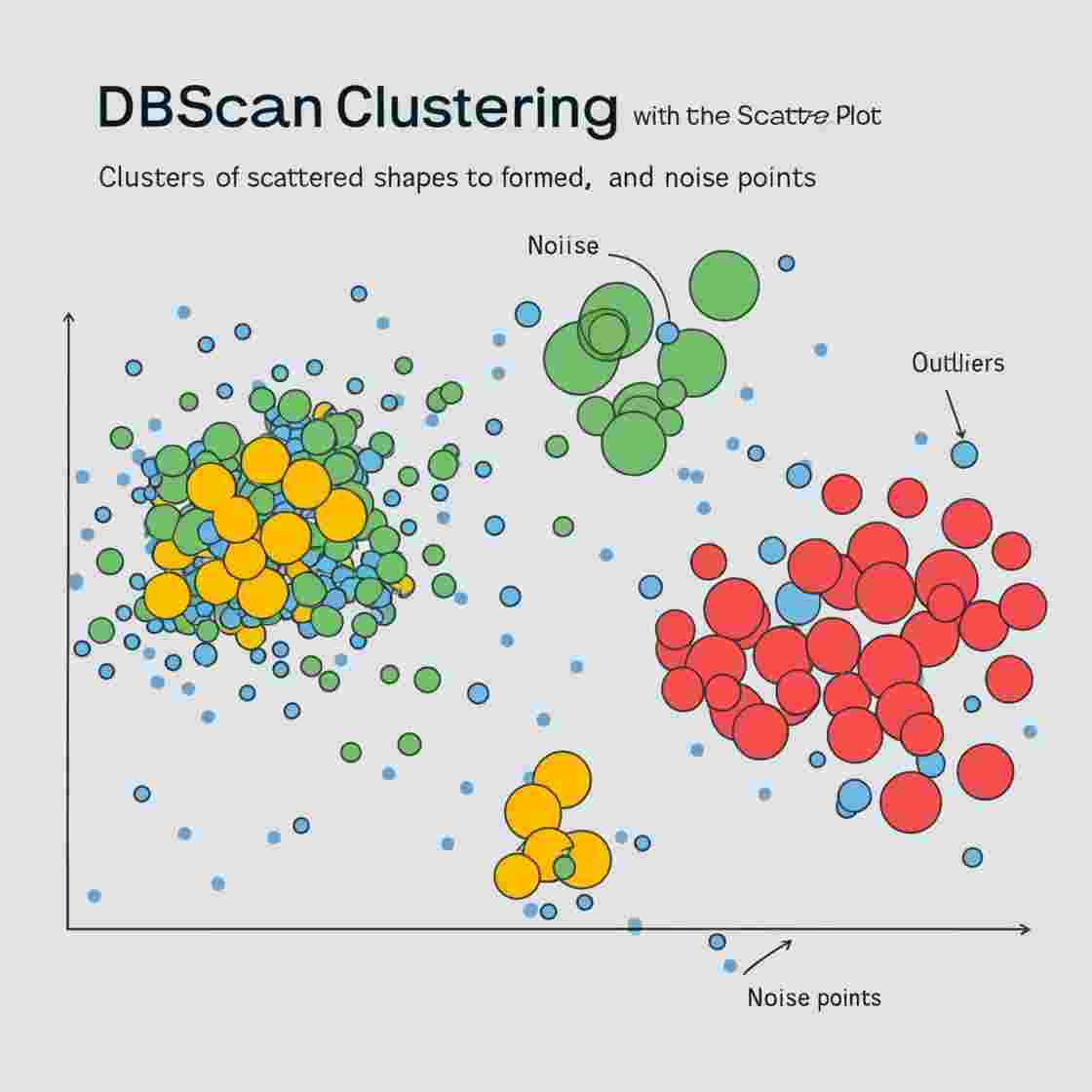
DBSCAN classifies points into three categories:
- Core Points:
Points with at least a minimum number of neighboring points (defined bymin_samples) within a specified distance (eps). Core points are the backbone of clusters. - Border Points:
Points that are within theepsdistance of a core point but do not themselves have enough neighbors to be core points. They are part of the cluster but are on its boundary. - Noise Points:
Points that do not belong to any cluster because they are too far from any core points. These are considered outliers or noise.
Advantages of DBSCAN
- No Need to Specify the Number of Clusters: DBSCAN automatically determines the number of clusters based on the density distribution, unlike K-Means, which requires specifying
k. - Robust to Noise and Outliers: DBSCAN can handle noise effectively, labeling outliers separately, which is useful for real-world messy datasets.
- Handles Arbitrary Cluster Shapes: DBSCAN is capable of detecting clusters with complex, non-linear shapes, making it suitable for datasets with irregular patterns.
Implementing DBSCAN with Scikit
To get started with DBSCAN Scikit-Learn, ensure you have the required libraries installed:
pip install scikit-learn matplotlib numpy pandas
Import the Libraries
We’ll begin by importing the necessary libraries:
import numpy as np

import matplotlib.pyplot as plt

from sklearn.cluster import DBSCAN

from sklearn.datasets import make_moons

from sklearn.preprocessing import StandardScaler
Generate or Load the Data
We’ll generate synthetic data using the make_moons function to demonstrate DBSCAN Scikit-Learn’s ability to handle non-linear clusters. The data will be standardized using StandardScaler.
# Generate synthetic data with two interlocking half-moons

X, y = make_moons(n_samples=500, noise=0.05)
# Standardize the data to have mean 0 and variance 1

X = StandardScaler().fit_transform(X)
Apply DBSCAN
Next, we’ll apply the DBSCAN algorithm by initializing it with the eps and min_samples parameters.
# Initialize DBSCAN with parameters eps=0.3 and min_samples=5

dbscan = DBSCAN(eps=0.3, min_samples=5)
# Fit the DBSCAN model to the data

dbscan.fit(X)
# Retrieve cluster labels for each data point

labels = dbscan.labels_
Visualize the Clusters
# Create a scatter plot of the data points colored by their cluster label

plt.scatter(X[:, 0], X[:, 1], c=labels, cmap='viridis')

plt.title("DBSCAN Clustering with Scikit-Learn")

plt.xlabel("Feature 1")

plt.ylabel("Feature 2")

plt.show()
Explanation of Parameters
eps: Defines the maximum distance between two points for one to be considered a neighbor of the other. Smaller values create tighter clusters, while larger values may merge distinct clusters.min_samples: Specifies the minimum number of points required to form a dense region (core point). Lower values increase sensitivity to noise, while higher values reduce it.
DBSCAN Scikit Learn: Understanding the Output
The labels_ attribute contains the cluster labels assigned to each data point:
- Positive integers represent different clusters (e.g., 0, 1, 2).
- -1 indicates noise points that do not belong to any cluster.
Customizing DBSCAN for Better Results
Tuning eps
Adjusting eps is critical for finding the right balance between forming too few or too many clusters. A small eps may lead to many small clusters, while a large eps may merge distinct clusters into one.
Adjusting min_samples
Increasing min_samples reduces the number of core points, making DBSCAN Scikit-Learn more conservative, which can help eliminate noise but may exclude valid clusters.
Real-World Example: Clustering the Iris Dataset
from sklearn.datasets import load_iris
# Load the Iris dataset

iris = load_iris()

X_iris = StandardScaler().fit_transform(iris.data)
# Apply DBSCAN to the Iris dataset

dbscan_iris = DBSCAN(eps=0.5, min_samples=5)

dbscan_iris.fit(X_iris)
# Retrieve cluster labels

labels_iris = dbscan_iris.labels_
# Count the unique clusters (excluding noise)

unique_clusters = np.unique(labels_iris)

print(f"Number of clusters: {len(unique_clusters) - 1}")
Visualizing the Clusters
plt.scatter(X_iris[:, 0], X_iris[:, 1], c=labels_iris, cmap='plasma')

plt.title("DBSCAN Clustering on Iris Dataset")

plt.xlabel("Feature 1")

plt.ylabel("Feature 2")

plt.show()
When to Use DBSCAN Scikit Learn
DBSCAN is ideal for:
- Datasets with noise or outliers.
- Clusters with irregular or arbitrary shapes.
- Scenarios where the number of clusters is unknown.
Limitations
- Sensitive to the choice of
epsandmin_samples. - Struggles with high-dimensional data due to the curse of dimensionality.
- Not well-suited for datasets with varying densities.
DBSCAN Scikit Learn : Conclusion
DBSCAN is a versatile and powerful clustering algorithm that excels at discovering clusters in noisy, complex datasets. DBSCAN Scikit-Learn provides a simple implementation that makes it accessible for data scientists and analysts. Understanding how to tune parameters like eps and min_samples is key to unlocking its full potential.

